Shared coefficients and shared baseline

This vignette is still an early draft.

1 Background

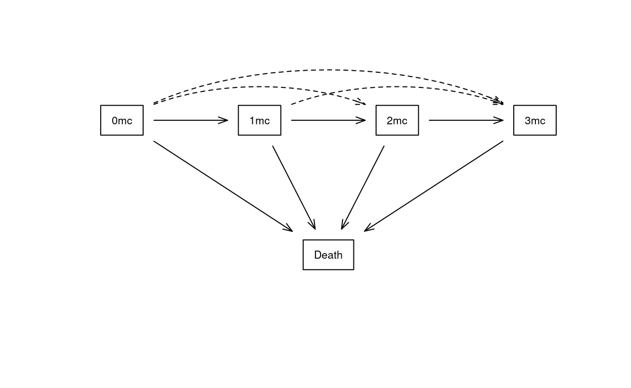
A multi-state hazards (MSH) model will model the transitions between multiple states. An example is analysis of the NAFLD data, whose transition diagram is shown in Figure 1; living patients will have 0–3 of the following metabolic comorbidities: diabetes, hypertension, and hyperlipidemia. In this figure there are 10 transitions (arrows). For any given pair of transitions a:b and c:d there are 6 different choices to organize the coefficients and baseline hazards, shown in Table 1. This document explores both technical and statistical aspects of those choices.

Table 1: Choices for any pair of transitions in a multistate model.

	Baseline hazard
	Separate	Proportional	Identical
Separate coefficients	1	2	3
Shared coefficients	4	5	6

2 Data

We will use two running examples in this document. The first is data on non-alcoholic liver disease (NAFLD) which is represented by the state space shown in Figure 1. Living subjects can have one or more of three metabolic comorbidities of diabetes, hypertension and hyperlipidemia. The study focuses on the impact of a NAFLD diagnosis on the rate at which subjects progress through the three states.

Figure 1: State space for the NAFLD data. The dashed lines are transitions that would not be observed if monitoring were continuous, but are present in the observed data.

Below is the transition table for the data set.
A direct transition from 0 to 3 of the comorbidities can not occur, biologically; no one aquires both hypertension and diabetes on the exact same second of the exact same day. We observe 4 such transitions, however, because our observation of any subject is intermittent. These “jump” transitions, the dotted lines in Figure 1, are a motivation for shared coefficient models.

> check1 <- survcheck(Surv(age1, age2, event) ~ nafld + male, data=ndata, 
                    id=id, istate=cstate)
> 
> check1$transitions

       to
from     1mc  2mc  3mc death (censored)
  0mc   1829   70    4   263       5705
  1mc      0 1843   28   243       4567
  2mc      0    0 1048   417       3687
  3mc      0    0    0   441       2220
  death    0    0    0     0          0

Figure 2: State space for the PBC example.

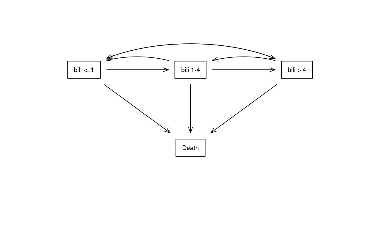
The primary biliary cholangitis state space is shown in Figure 2. The states in this example are created by categorization of the continuous bilirubin variable. Primary biliary cholangitis is an inflammatory disease, thought to be of auto-immune origin, characterized by a slow but inexhortable loss of the small bile ducts in the liver, as scar replaces functional tissue. Bilirubin and other markers of liver compromise rise slowly over time, then more quickly once the liver’s excess capacity has been exhausted. Figure 2 shows a multi-state model that includes bilirubin progression. Many of the reverse transitions (dotted lines in the figure) will be subjects whose true bilirubin value is currently near one of the cut points. There are very few observed jumps from normal bilirubin to \(>4\) or vice-versa (3 and 1, respectively).

3 Separate hazards

3.1 Separate coefficients

Separate coefficients and separate hazards for each transition is the default for a multi-state hazards (MSH) model using . The code below uses the NAFLD data.

> nfit1 <- coxph(Surv(age1, age2, event) ~ nafld + male, data = ndata,
                id = id, istate = cstate)

Warning in agreg.fit(X, Y, istrat, offset, init, control, weights =
weights, : Loglik converged before variable 8 ; beta may be infinite.

> round(coef(nfit1, matrix=TRUE), 2)

       1:2  1:3  2:3   1:4  2:4  3:4  1:5  2:5  3:5  4:5
nafld 0.93 0.31 0.53  1.51 0.08 0.48 0.63 0.53 0.55 0.06
male  0.16 0.54 0.25 12.80 0.02 0.15 0.43 0.47 0.36 0.16
attr(,"states")
[1] "0mc"   "1mc"   "2mc"   "3mc"   "death"

The fit has given a warning about a potentially infinite coefficient. Indeed, a look at the coefficient matrix shows a value of 12.8 for male sex, for the 1:4 (0MC to 3MC) transition, exp(12.8) \(> 362000\) which is effectively infinite for a sample of 17 thousand subjects, and the log partial likelihood had not yet reached its maximum. Further checking shown below identifies that 0/4246 female and 4/3675 males who were “at risk” for a 0mc:3mc jump had such an event, the hazard ratio for male sex is \(.001/0 = \infty\). We will address this issue in Section 3.2.

> temp <- with(subset(ndata, cstate=="0mc"), table(event, male))
> temp <- rbind(temp, Total= colSums(temp))
> temp

            0    1
censored 3152 2603
1mc       937  892
2mc        30   40
3mc         0    4
death     127  136
Total    4246 3675

The underlying coxph code fits all 10 of the transitions in model nfit1 simultaneously by creating a stacked data set. Two internal matrices cmap and smap direct the setup of the computation.

> ## internal mapping matrices
> nfit1$cmap

      1:2 1:3 2:3 1:4 2:4 3:4 1:5 2:5 3:5 4:5
nafld   1   3   5   7   9  11  13  15  17  19
male    2   4   6   8  10  12  14  16  18  20

> nfit1$smap

           1:2 1:3 2:3 1:4 2:4 3:4 1:5 2:5 3:5 4:5
(Baseline)   1   2   3   4   5   6   7   8   9  10

> 
> ## number of data rows in each state
> table(ndata$cstate)

 0mc  1mc  2mc  3mc 
7921 6764 5249 2749 

The cmap and smap matrices are used by the internal stacker routine to create expanded data used for the partial likelihood solution. The result has an expanded X, Y and transition variables which contain first all the data rows for transition 1 (0mc:1mc, 7921 rows), then for transition 2 (0mc:2mc, 7921 rows, etc. up to transition 10 (3mc:death, 2749 rows). The transition variable has repeated values of 1, 1, … , 1, 2, … , 2, 3, … 10. The first block of the expanded Y has a simple 0/1 status with 1 for a transition from 0mc to 1mc for the observations in that block. The expanded X matrix is block diagonal for this fit, as shown in Equation 1. Here \(X^{(1)}\) is all the rows of the data that are at risk for the first transtion (7921 rows, 2 columns), and etc. to \(X^{(10)}\) for the tenth transition. The final matrix has 20 columns, one for each coefficient, and 65223 rows. The 20 coefficients for the 10 transitions are now fit all at once using a single call to the internal Cox model fitting routine agreg.fit, with the transition as a strata.

\[ \begin{equation} \left( \begin{array}{cccc} X^{(1)} &0 & \ldots & 0 \\ 0 & X^{(2)} & \ldots & 0 \\ 0 & \vdots & \ddots & \vdots \\ 0 & 0 & 0 & X^{(10)} \end{array} \right) \end{equation} \tag{1}\]

3.2 Shared coefficients

You will have noticed that nfit1 gave a warning message that coefficient 8 appears to be infinite, which is the estimated male effect for the 1:4 transition. There are only 4 0mc to 3mc transitions in the data, and all of them are males, so indeed the MLE solution is \(\hat \beta= \infty\); there simply are not enough events in this stratum to estimate 2 coefficients. The other two jumps of Omc:2mc and 1mc:3mc also have small counts.

Biologically, we know that acquisition of 2 new comorbidities on the same exact day does not actually happen. An alternative model is to have coefficients for an increase from 0mc to “one or more” and from 1mc to “two or more”. This is shown below.

> nfit2 <- coxph(list(Surv(age1, age2, event) ~ nafld + male,
                     1:2 + 1:3 + 1:4 ~ nafld + male / common,
                     2:3 + 2:4 ~ nafld + male/common),
                data=ndata, id= id, istate= cstate)
> nfit2$cmap

      1:2 1:3 2:3 1:4 2:4 3:4 1:5 2:5 3:5 4:5
nafld   1   1   3   1   3   5   7   9  11  13
male    2   2   4   2   4   6   8  10  12  14

> 
> round(coef(nfit2, matrix=TRUE), 2)

       1:2  1:3  2:3  1:4  2:4  3:4  1:5  2:5  3:5  4:5
nafld 0.91 0.91 0.52 0.91 0.52 0.48 0.63 0.53 0.55 0.06
male  0.18 0.18 0.25 0.18 0.25 0.15 0.43 0.47 0.36 0.16
attr(,"states")
[1] "0mc"   "1mc"   "2mc"   "3mc"   "death"

When the model formula is a list of formulas, the first formula is the default for all transtions and subsequent lines amend that formula for selected transtions. Variables can be add or removed in the same way as update.formula. The common modifier signals common coefficients for these variables and transitions.

The final model has 14 coefficients instead of 20, and the overall risk of exp(.18) = 1.2 for males for the 0:mc to 1+ transition is much more sensible. The expanded X matrix in this model will have the same number of rows as before, but 14 rather than 20 columns. It is no longer block diagonal, column 1 for instance now has non-zero entries in 3 different transition blocks.

The coefficient vector found in the fit object has 14 unique entries and the estimated variance/covariance matrix is 14 by 14, these are what are returned by the coef and vcov functions. These choices make the MSH model results better fit in to the standard Cox model framework. The matrix=TRUE modifier for coef gives a more user friendly printout.

3.3 Predicted values

For predicted values from a MSH model, we will normally want to show separate predictions for each transition. For linear predictors, this is facilitated by the matrix argument to coef.coxphms and vcov.coxphms, the MSH methods for the coef and vcov methods. For example

> eta2 <- model.matrix(nfit2) %*% coef(nfit2, matrix=TRUE)
> dim(eta2)

[1] 22683    10

> nrow(ndata)

[1] 22683

> 
> v2 <- vcov(nfit2, matrix=TRUE)
> dim(v2)

[1] 14 14

The model.matrix function for the fit returns the standard X matrix, which is the correct object for this task, not the expanded one which was needed (temporarily) for computing the fit. Then eta2 is a matrix with one row for each observation in the data set and one column for each transition. This matrix contains more values than we need, formally. Observation 1 is a row with current state of cstate = 0mc, for instance, so one could argue that the 2mc:death entry of row 1 is not ``relevant’’ to that row of the data.

Predicted probability in state curves, however, are always for a hypothetical subject, in which case we do want all the predicted hazards, since all the hazards are needed to compute absolute risks. Remember that a predicted curve is for a particular subject (covariate values) at a particular time (age) in a particular starting state. We find it helpful to use the mental picture of “prediction for the patient currently sitting across from me in the examination room”, i.e., absolute prediction is always specific. For an ordinary alive/dead KM where everyone starts at time 0 we don’t have to think about starting state and starting time, but for multistate they are necessary.

> # predicted curves for a 50 year old female with and without NAFLD, who
> #  starts with none of the comorbidities.  Solid= NAFLD.
> dummy <- data.frame(nafld= 0:1, male=0)
> pstate2 <- survfit(nfit2, newdata=dummy, start.time=50, p0=c(1,0,0,0,0))
> plot(pstate2, col=rep(1:5, each=2), lty=1:2, lwd=2,
      xlab="Age", ylab="Probability in state")
> legend(70, 1, c("0mc", "1mc", "2mc", "3mc", "death"), col=1:5, lty=1, lwd=2,
        bty='n')

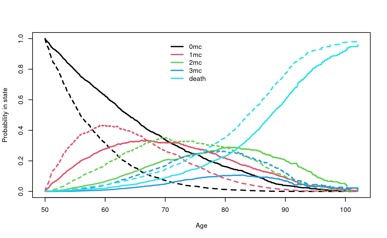
(Yet to do: show examples with predict())

4 Shared proportional hazards

An alternative to separate hazards is shared proportional hazards. We will separate this into three cases: “common endpoint” will be pairs of transitions such as A:C and B:C that lead to a common state, “disjoint” a pair like A:C and B:D, and “common origin” A:B and A:C.

4.1 Common endpoint

This has been by far the most prevalent example in our work. As an example, we might assume that the 4 transitions from comorbidity to death, in the NAFLD data, have the same shape but a different scale. That is

\[ \begin{align} \lambda_{1d}(t,x) &= \lambda_{0d}(t) \exp(\gamma_1)\exp(X\beta_{.8}) \label{nshare1}\\ \lambda_{2d}(t,x) &= \lambda_{0d}(t) \exp(\gamma_2)\exp(X\beta_{.9}) \label{nshare2} \\ \lambda_{3d}(t,x) &= \lambda_{0d}(t) \exp(\gamma_3)\exp(X\beta_{.10}) \label{nshar3}\\ \end{align} \]

where \(\lambda_{kd}\) is the hazard for \(k\) comorbidities to death, and we have selected the appropriate column of the coefficient matrix \(\beta\). (For both nfit1 and nfit2 the matrix form has has 10 columns, 1 per transition, with the last 4 being the transitions to death.)

Here is sample code to fit this model, retaining the shared coefficients for mc:mc transition used in nfit2. Behind the scenes, the code bundles the \(\gamma\) and \(\beta\) coefficients together, in order to jointly estimate both of them using the agreg.fit routine. We take advantage of the use of “1” as the representation of an intercept in the formula modeling language of R, along with the fact that the basline hazard can be thought of as the “intercept” term of a MSH model, to create a compact notation. Our call has only one more line than nfit2.

> nfit3 <- coxph(list(Surv(age1, age2, event) ~ nafld + male,
                     1:2 + 1:3 + 1:4 ~ nafld + male / common,
                     2:3 + 2:4 ~ nafld + male/common,
                     0:5  ~ cstate + 1 / common), 
                data=ndata, id= id, istate= cstate)
> print(nfit3, digits=2)

Call:
coxph(formula = list(Surv(age1, age2, event) ~ nafld + male, 
    1:2 + 1:3 + 1:4 ~ nafld + male/common, 2:3 + 2:4 ~ nafld + 
        male/common, 0:5 ~ cstate + 1/common), data = ndata, 
    id = id, istate = cstate)

             
1:2, 1:3, 1:4  coef exp(coef) se(coef) robust se    z      p
        nafld 0.915     2.496    0.063     0.067 13.6 <2e-16
        male  0.179     1.196    0.046     0.048  3.7  2e-04

        
2:3, 2:4  coef exp(coef) se(coef) robust se   z      p
   nafld 0.521     1.683    0.052     0.056 9.3 <2e-16
   male  0.246     1.278    0.047     0.050 4.9  9e-07

       
3:4      coef exp(coef) se(coef) robust se   z     p
  nafld 0.485     1.624    0.065     0.068 7.1 9e-13
  male  0.149     1.161    0.063     0.065 2.3  0.02

           
1:5          coef exp(coef) se(coef) robust se    z     p
  nafld      0.53      1.70     0.22      0.22  2.4  0.01
  male       0.41      1.51     0.12      0.12  3.4 6e-04
  cstate1mc -0.30      0.74     0.13      0.13 -2.4  0.02
  cstate2mc -0.18      0.84     0.12      0.12 -1.5  0.13
  cstate3mc  0.62      1.86     0.12      0.12  5.1 4e-07

           
2:5          coef exp(coef) se(coef) robust se    z     p
  nafld      0.51      1.66     0.15      0.15  3.4 6e-04
  male       0.47      1.59     0.13      0.13  3.7 2e-04
  cstate1mc -0.30      0.74     0.13      0.13 -2.4  0.02
  cstate2mc -0.18      0.84     0.12      0.12 -1.5  0.13
  cstate3mc  0.62      1.86     0.12      0.12  5.1 4e-07

           
3:5           coef exp(coef) se(coef) robust se    z     p
  nafld      0.571     1.771    0.104     0.107  5.3 9e-08
  male       0.364     1.438    0.098     0.099  3.7 2e-04
  cstate1mc -0.300     0.741    0.133     0.127 -2.4  0.02
  cstate2mc -0.175     0.839    0.121     0.117 -1.5  0.13
  cstate3mc  0.618     1.856    0.123     0.122  5.1 4e-07

           
4:5           coef exp(coef) se(coef) robust se    z     p
  nafld      0.128     1.136    0.098     0.101  1.3  0.21
  male       0.160     1.173    0.096     0.099  1.6  0.11
  cstate1mc -0.300     0.741    0.133     0.127 -2.4  0.02
  cstate2mc -0.175     0.839    0.121     0.117 -1.5  0.13
  cstate3mc  0.618     1.856    0.123     0.122  5.1 4e-07

 States:  1= 0mc, 2= 1mc, 3= 2mc, 4= 3mc, 5= death 

Likelihood ratio test=566  on 17 df, p=<2e-16
n= 22683, unique id= 17549, number of events= 6186 

Since the current state of each observation is a factor variable cstate, the default coding for factors in R does exactly what we wished. We see that after adjustment for sex and NAFLD status, those with 3 comorbidities have a higher death rate than 0mc, which is not a surprise, but also that 1mc appears to be lower than 0mc. More on that will be discussed further below.

One aspect of the printout which is potentially misleading is that all 3 cstate coefficients appear for all 4 transitions. However, for the 1:5 transition (0mc:death) the three 0/1 dummy variables cstate1mc, cstate2mc and cstate3mc will all be 0. The coefficients that appear in the 1:5 printout above will never be used. For the 2:5 transition only cstate1mc is non-zero so the cstate2mc and cstate3mc coefficients are redundant, with similar comments for the 3:5 and 4:5 transtions. We can fit an equivalent model with somewhat simpler printout by creating a single 0/1 dummy variable which is 0 only for the 0mc state.

> ndata$notzero <- 1*(ndata$cstate != "0mc")
> nfit3b <- coxph(list(Surv(age1, age2, event) ~ nafld + male,
                     1:2 + 1:3 + 1:4 ~ nafld + male / common,
                     2:3 + 2:4 ~ nafld + male/common,
                     c(2,3,4):5 ~ notzero,
                     0:5  ~ 1 / common), 
                data=ndata, id= id, istate= cstate)
> round(coef(nfit3b, matrix=TRUE), digits=2)

         1:2  1:3  2:3  1:4  2:4  3:4  1:5   2:5   3:5  4:5
nafld   0.91 0.91 0.52 0.91 0.52 0.48 0.53  0.51  0.57 0.13
male    0.18 0.18 0.25 0.18 0.25 0.15 0.41  0.47  0.36 0.16
notzero 0.00 0.00 0.00 0.00 0.00 0.00 0.00 -0.30 -0.18 0.62
attr(,"states")
[1] "0mc"   "1mc"   "2mc"   "3mc"   "death"

> 
> all.equal(nfit3$loglik, nfit3b$loglik)

[1] TRUE

Another approach which provides an even clearer printout is to use the shared option.

> nfit3c <- coxph(list(Surv(age1, age2, event) ~ nafld + male,
                     1:2 + 1:3 + 1:4 ~ nafld + male / common,
                     2:3 + 2:4 ~ nafld + male/common,
                     0:5 ~ nafld + male/ shared),
                data=ndata, id= id, istate= cstate)
> 
> round(coef(nfit3c, matrix=TRUE), 2)

         1:2  1:3  2:3  1:4  2:4  3:4  1:5   2:5   3:5  4:5
nafld   0.91 0.91 0.52 0.91 0.52 0.48 0.53  0.51  0.57 0.13
male    0.18 0.18 0.25 0.18 0.25 0.15 0.41  0.47  0.36 0.16
ph(1:5) 0.00 0.00 0.00 0.00 0.00 0.00 0.00 -0.30 -0.18 0.62
attr(,"states")
[1] "0mc"   "1mc"   "2mc"   "3mc"   "death"

> all.equal(nfit3c$loglik, nfit3$loglik)

[1] TRUE

We stated earlier that the baseline hazard plays the role of an intercept, and it does so in another way that is less often noticed. In a linear model, the intercept term makes a fit invariant to simple changes in the covariates, e.g., replace some covariate \(x\) in model with \(z= x+2\), and the predicted values \(\hat y\) from the fit will remain unchanged, as do all of the non-intercept coefficients and their estimated standard errors. A much more common case is replacement of a 0/1 covariate with 1/0, e.g., one fit coded 1=male and another 1=female. Compare the coefficients of the modified model below. Nothing changes except the ph(1:5) coefficients, and they do they shift by a constant. This means that we must be cautious about interpreting the absolute values of these coefficients, and perhaps even more so any p-values, just as would be the case for intercepts in a linear model.

> ndata$male23 <- ndata$male + 2  # code male as 2/3
> nfit3d <- coxph(list(Surv(age1, age2, event) ~ nafld + male23,
                     1:2 + 1:3 + 1:4 ~ nafld + male23 / common,
                     2:3 + 2:4 ~ nafld + male23/common,
                     0:5 ~ nafld + male23/ shared),
                data=ndata, id= id, istate= cstate)
> 
> round(coef(nfit3c, matrix=TRUE), 2)

         1:2  1:3  2:3  1:4  2:4  3:4  1:5   2:5   3:5  4:5
nafld   0.91 0.91 0.52 0.91 0.52 0.48 0.53  0.51  0.57 0.13
male    0.18 0.18 0.25 0.18 0.25 0.15 0.41  0.47  0.36 0.16
ph(1:5) 0.00 0.00 0.00 0.00 0.00 0.00 0.00 -0.30 -0.18 0.62
attr(,"states")
[1] "0mc"   "1mc"   "2mc"   "3mc"   "death"

> 
> round(coef(nfit3d, matrix=TRUE), 2)

         1:2  1:3  2:3  1:4  2:4  3:4  1:5   2:5   3:5  4:5
nafld   0.91 0.91 0.52 0.91 0.52 0.48 0.53  0.51  0.57 0.13
male23  0.18 0.18 0.25 0.18 0.25 0.15 0.41  0.47  0.36 0.16
ph(1:5) 0.00 0.00 0.00 0.00 0.00 0.00 0.00 -0.41 -0.08 1.12
attr(,"states")
[1] "0mc"   "1mc"   "2mc"   "3mc"   "death"

However, just as in a linear model, this shift does not affect absolute predictions. We point out the following about the predicted survival curves:

1. A predicted curve needs to have a starting time, a starting state, and the covariate values of the hypothetical subject.
2. Covariates associated with the \(\gamma\) coefficients are not a part of newdata. This is because those coefficients belong to the state, not to the covariates of the hypothetical subject.

> dummy$male23 <- dummy$male + 2
> pstate3c <- survfit(nfit3c, newdata=dummy, start.time=50, p0=c(1,0,0,0,0))
> pstate3d <- survfit(nfit3d, newdata=dummy, start.time=50, p0=c(1,0,0,0,0))
> all.equal(pstate3c$pstate, pstate3d$pstate)

[1] TRUE

The survfit routine recognizes \(\gamma\) coefficients in the model by their special variable name ph(1:5). (I have little doubt that someone, somewhere will eventually create a variable name enough like this to fool my code, and then post it as a bug.) For probability in state curves based on model nfit3b a bit more is needed: the variable notzero looks, to the survfit code, no different than any other; the routine needs the user’s help to identify that this variable is associated with \(\gamma\) rather than \(\beta\) terms. At this time, the method is to add notzero to the dummy data set with a value of NA. From a user interface perspective simply leaving notzero out of the dummy data set would be cleaner, but the model.matrix routine from base R, which I depend on, is unhappy if a variable found in the model formula is missing from newdata. I don’t yet have a way to work around that.

To do: example using nfit3b, once I have the NA code debugged. To do: add the PBC example.

4.2 Risk sets

One aspect of this that we have not mentioned is that with a set of transitions A:D + B:D + C:D to a common final state, the risk sets also make sense. Since no subject can be two places at once (in two states at the same time), the risk set for the shared hazard at time \(t\) = (in state A at \(t\)) + (in state B at \(t\)) + (in state C at \(t\)) will have no duplicate subjects. The Cox partial likelihood term for an event at \(t\) will thus have a proper denominator, i.e., a weighted sum over all those at risk, where \(\exp(X\hat \beta)\) are the risk weights. This identity of risk sets is what makes it particularly easy to jointly estimate \(\gamma\) and \(\beta\).

4.3 Shared hazards, common starting state

This is the case where a pair of transitions A:B and A:C are considered to have a common hazard shape. At this point:

• We have not encountered any examples where such an assumption makes biological sense. Without a concrete example, it has not been possible to reason out what the software should do in this case.
• The current code will create risk sets with multiple copies of the same subject. We are not at all sure that this makes sense, in fact we rather doubt it. (Exception, no duplicates are created if A:B and A:C have common coefficients for all variables.)

If any reader has such a use case we would be delighted to hear of it.

4.4 Shared hazard, disjoint pairs

The second subcase is a shared baseline hazard for a transition pair like A:B and C:D. In general, it may be hard to think of situations where we would be willing to assume that these two transitions, to two disparate endpoints B and D, would have hazards of the same shape. We have encountered one example, however, which has motivated the details in our code. It can be seen as an extension of the PBC example.

To do: This is not yet reliably working in our code.

5 Identical hazards

Identical hazards are a problem child. The issue is that such models will be at the mercy of how covariates are coded. As a simple case, consider the NAFLD data, and assume that the transitions to death have an identical hazard rather than a proportional one. It turns out that the impact of changing the coding of male sex from 0/1 to 2/3 is profound, with a different log-likelihood and multiple coefficient changes.

> nfit4a <- coxph(list(Surv(age1, age2, event) ~ nafld + male, 
                      1:2 + 1:3 + 1:4 ~ nafld + male/common, 
                      2:3 + 2:4 ~ nafld + male/common, 
                      0:5 ~ 1/common),
                 data = ndata, id = id, istate = cstate)
> nfit4b <- coxph(list(Surv(age1, age2, event) ~ nafld + male23, 
                      1:2 + 1:3 + 1:4 ~ nafld + male23/common, 
                      2:3 + 2:4 ~ nafld + male23/common, 
                      0:5 ~ 1/common),
                 data = ndata, id = id, istate = cstate)
> 
> temp <- rbind(male01= nfit4a$log, male23= nfit4b$log)
> colnames(temp) <- c("Initial loglik", "Final loglik")
> temp

       Initial loglik Final loglik
male01      -40534.77    -40284.86
male23      -40534.77    -40260.73

> 
> plot(coef(nfit4a), coef(nfit4b), xlab="Coefficients, model with male as 0/1",
      ylab= "Coefficients, male as 2/3")
> abline(0,1)

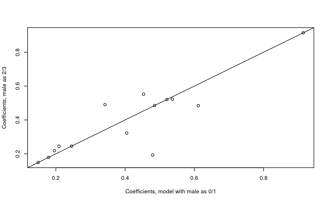
Many discussions mention a “common hazard function” as a modeling idea, but few have followed through on the consequences of assuming that \(\gamma =1\) uniformly.
If we also force common coefficients for all the covariates then the problem goes away, but that becomes, in essence, a single transition model of “either outcome”.

Speculation:

• The same sort of confusions occur in linear models with regression through the origin. I don’t know if that analogy is helpful, however.
• I think that part of the problem above is that the overall death rate for 3mc:death is substantially higher than 0mc:death, and so any other variable that is out of balance will get recruited as an alias for the missing \(\gamma\) coefficient. NAFLD prevalence, for instance, is .89 for the 0mc stratum and .56 for the 3mc stratum.